January 1, 0001
ABSTRACT
A dataset obtained from Kaggle on the concentrations of Cs-137, Cs-134, and I-131 in the air following the Chernobyl Nuclear Power Plant disaster was used to look at how mean Cs-137 concentrations differed across countries in Europe. Peer reviewed research has shown factors such as prevailing winds and varying levels of precipitation across Europe affected how radioactive fallout was distributed across the continent. Statistical analysis was conducted to show there was a significant difference between the mean concentrations of Cs-137 in Austria when compared to Czechoslovakia even though both countries have almost identical longitudes and neighbor each other.
INTRODUCTION
On April 26, 1986 reactor #4 of the Chernobyl Nuclear Power Plant in Ukraine released a large amount of energy as the core exploded after being put into an unstable condition. Many professionals regard this event as the most devastating nuclear disaster of all time and the event consequently led to the downfall of the Soviet Union. As the radioactive fallout quickly spread throughout Europe inhabitants living closest to the site of explosion including families, farmers, powerplant workers, and wildlife were affected by the radioactive contamination. At the time of the accident there was a lack of equipment present to record data concerning the dosage of radiation these inhabitants received, but tooth enamel was later used to determine that they potentially received 6-8 times the dose of lethal radiation (Petryna, 2013). For this inquiry I decided it would be interesting to explore how countries across Europe were affected by the Chernobyl disaster and quantify this based on how the concentrations of Cs-137 varied across these recorded areas.
After investigating peer reviewed research, I found the areas that had greater amounts of precipitation following the disaster such as parts of Austria also exhibited higher concentrations of Cs-137 despite being further away from the exclusion zone than other countries (Bossew, Ditto, Falkner, Henrich, Kienzl, and Rappelsberger, 2001). These storms led to radioactive fallout being transported in a way that did not exclusively represent a contamination gradient growing weaker the further away areas were from the power plant. The varying precipitation across Europe led to the depth underground radioactive fallout was able to be deposited into the soil and the prevailing winds also worked to distribute the contamination (Zablotska, 2016). This had effects on existing ecosystems as the contamination was able to be recycled time and time again with organisms such as higher fungi, mosses, and lichens better able to take up Cs-137 (Avery, 1996). This is a major reason why cleanup efforts to cover and take away contaminated soil were made, as inhalation of the nuclear fallout is a concern for life on Earth. The many Chernobyl liquidators that put their health and lives on the line to combat an unforeseen and complex problem deserve a special thanks. If it were not for their dedication and hard work the immediate and distant factors following the Chernobyl disaster would have been even more devastating.
DATA
I stumbled upon a dataset on Kaggle as I was looking for something to explore for Inquiry 3. The Chernobyl dataset included information on different concentrations of radioactive isotopes measured across different localities of Europe following the disaster. The isotopes recorded were Cs-137, Cs-134, and I-131. Cs-137 was a focus for scientists as it has a longer half-life of 30.2 years compared to the other isotopes Cs-134 and I-131 only having half-lives of 2.06 years and 8 days respectively. Cs-137 offered scientists contamination levels that were easier to detect and measure in the field. The data was extracted from the REM data bank at CEC Joint Research Centre Ispra and also contains information such as locality, country, latitude, longitude, date, and duration of sampling.
I used R Studio to import the data obtained from Kaggle to see there were 2051 observations across 11 variables. The data was then cleaned of NAs and blank cells leaving 1533 observations. I removed two observations that had the letter “L” as a value in the Cs-137 column as I could not find the notation pertaining to what this letter meant. The cells that contained the less than symbol (<) were replaced with zeroes as the data recorded was below the detectable limit for either of the three radioactive isotopes. Lastly, I was obtaining errors when trying to obtain various summary statistics from the measurements as the output kept insisting the argument was not numerical or logical. I fixed this issue by coding all the measurements as characters and then again as numeric.
air <- air %>% na_if("") %>% na.omit  #omit rows with blanks
air <- air %>% na_if("N") %>% na.omit  #omit rows with NAs
air <- air %>% na_if("L") %>% na.omit  #omits rows with unknown character L
air[air == "<"] <- 0  #replace '<' entries representing less than the measurable limit with 0
air$Cs.137..Bq.m3. <- as.numeric(as.character(air$Cs.137..Bq.m3.))
air$Cs.134..Bq.m3. <- as.numeric(as.character(air$Cs.134..Bq.m3.))
air$I.131..Bq.m3. <- as.numeric(as.character(air$I.131..Bq.m3.))
ANALYSIS
It can be seen after using the ‘n_distinct’ dplyr function that there are 15 distinct countries in the dataset. I thought it would be nice to then see what the max reported values for Cs-137 were across these different countries where data was collected. It was interesting to see that Poland was not included in data collection as it borders Ukraine serving as its immediate neighbor to the west. However, there was data on (formerly) Czechoslovakia, which borders part of Ukraine as well as Poland. Due to this I initially thought there would be high measurements of Cs-137 recorded from Czechoslovakia, but this was not found anywhere in the top 15 highest readings. Countries that appeared in the max the most included Germany and Austria, each with six entries. The highest recorded measurement oddly came from Nurmijaervi, Finland and I decided the next best way to visualize the data would be to obtain summary statistics on the mean, standard deviation, standard error, and counts for each country. I included the text output along with a ggplot to better visualize how many entries each country has in the dataset.
air %>% select(PAYS) %>% n_distinct()## [1] 15air %>% select(PAYS, Ville, Cs.137..Bq.m3.) %>% top_n(15, Cs.137..Bq.m3.) %>%
arrange(desc(Cs.137..Bq.m3.))## PAYS Ville Cs.137..Bq.m3.
## 1 FI NURMIJAERVI 11.900000
## 2 DE BROTJACKLRIEGEL 11.100000
## 3 DE NEUHERBERG 9.200000
## 4 DE BROTJACKLRIEGEL 8.800000
## 5 DE NEUHERBERG 7.500000
## 6 AU LINZ 6.648881
## 7 AU LINZ 6.500503
## 8 AU LINZ 6.165024
## 9 DE KARLSRUHE 5.900000
## 10 AU LINZ 5.452143
## 11 F VERDUN 5.400000
## 12 AU GRAZ 5.291000
## 13 DE KARLSRUHE 5.200000
## 14 AU LINZ 5.098655
## 15 NL DELFT 5.000000airsums <- air %>% group_by(PAYS) %>% dplyr::summarize(mean_Cs137 = mean(Cs.137..Bq.m3.),
sd_Cs137 = sd(Cs.137..Bq.m3.), count_Cs137 = n(), se_Cs137 = sd_Cs137/sqrt(count_Cs137)) %>%
print()## # A tibble: 15 x 5
## PAYS mean_Cs137 sd_Cs137 count_Cs137 se_Cs137
## <fct> <dbl> <dbl> <int> <dbl>
## 1 AU 0.984 1.44 157 0.115
## 2 BE 0.218 0.670 40 0.106
## 3 CH 0.422 0.510 34 0.0875
## 4 CZ 0.370 0.766 34 0.131
## 5 DE 0.707 1.62 186 0.119
## 6 ES 0.0131 0.0291 44 0.00439
## 7 F 0.212 0.602 180 0.0449
## 8 FI 0.487 2.09 33 0.363
## 9 GR 0.433 0.916 58 0.120
## 10 HU 0.432 0.458 13 0.127
## 11 IT 0.661 0.719 283 0.0427
## 12 NL 0.840 1.26 107 0.122
## 13 NO 0.215 0.619 73 0.0724
## 14 SE 0.0777 0.246 211 0.0170
## 15 UK 0.0899 0.319 78 0.0362ggplot(data = airsums, mapping = aes(x = reorder(PAYS, count_Cs137),
count_Cs137)) + geom_bar(stat = "identity") + scale_y_continuous(breaks = c(0,
25, 50, 75, 100, 125, 150, 175, 200, 225, 250, 275, 300)) +
ggtitle("Country Counts") + xlab("Country") + ylab("Count") +
theme_bw(base_size = 12)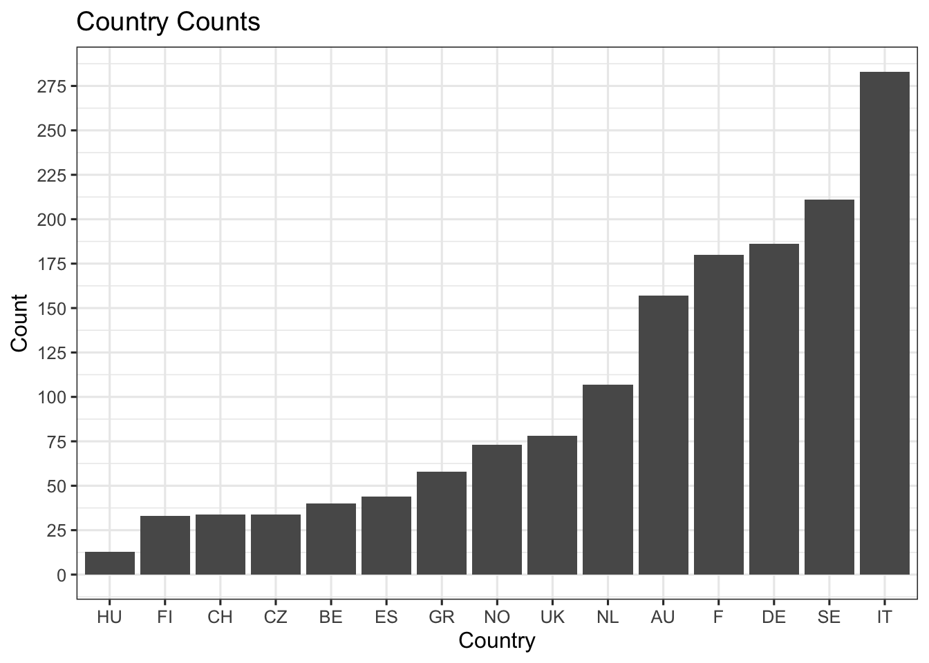 The data shows that Finland had the second lowest count amongst the 15 countries. Due to the relatively low number of observations compared to countries like Italy, Spain, and Germany it also had the highest standard deviation because of an observation of 11.9 Bq/m3 for Cs-137. It almost appears this could be an outlier especially since the neighboring Scandinavian country of Sweden with 211 observations reported a mean Cs-137 measurement of 0.077 Bq/m3. Now to visualize how these countries rank against each other for mean concentrations of Cs-137 I made a plot with standard error bars for each country.
ggplot(data = airsums, mapping = aes(x = reorder(PAYS, mean_Cs137),
mean_Cs137)) + geom_bar(stat = "identity") + geom_errorbar(aes(y = mean_Cs137,
ymin = mean_Cs137 - se_Cs137, ymax = mean_Cs137 + se_Cs137)) +
ggtitle("Mean Cs-137 Measurments") + xlab("Country") + ylab("Mean Cs-137 (Bq/m3") +
theme_bw(base_size = 12)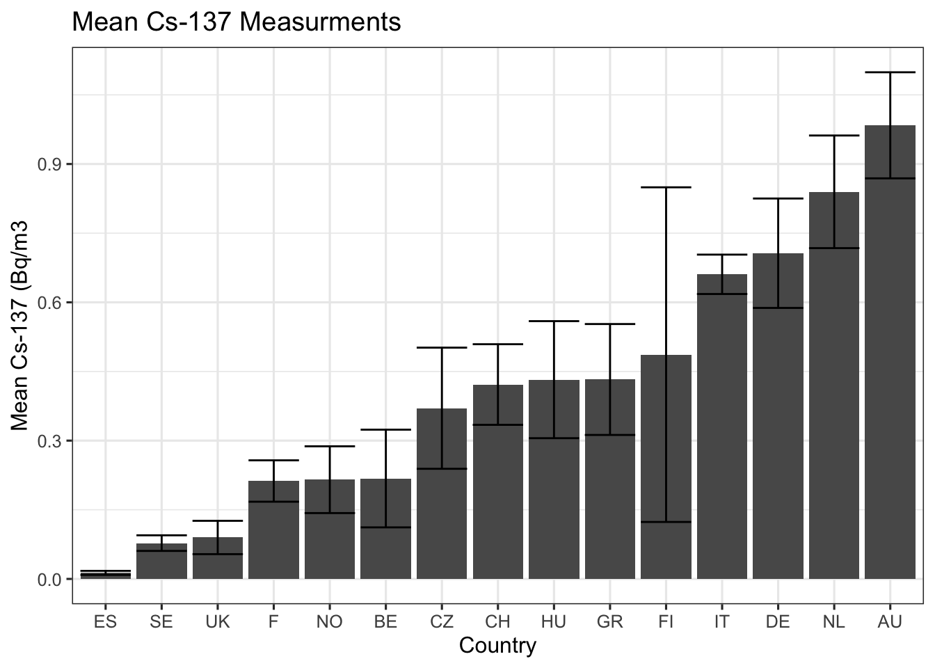 It was fascinating to note that the average measurement of Cs-137 in Austria was about twice that of Czechoslovakia despite the proximity to Ukraine. Take a look at the amount of observations for the locality Kosice (modern day eastern Slovakia). I expected to see some higher measurements of Cs-137 in Kosice, CZ (latitude: 21.25 degrees, longitude: 48.73 degrees) than Linz, AU (latitude: 14.30 degrees, longitude: 48.31 degrees) since they nearly have the same longitude. However, this was not the case as Kosice only showed a mean value of 0.390 Bq/m3 for Cs-137 (n=27) while Linz showed 2.056 Bq/m3 (n=43).
kosicecs137 <- air %>% select(PAYS, Ville, Cs.137..Bq.m3., Date) %>%
    filter(PAYS == "CZ", Ville == "KOSICE")
kosicecs137 %>% summarize(mean(Cs.137..Bq.m3.), sd(Cs.137..Bq.m3.))
## mean(Cs.137..Bq.m3.) sd(Cs.137..Bq.m3.)
## 1 0.3903704 0.8395619linzcs137 <- air %>% select(PAYS, Ville, Cs.137..Bq.m3., Date) %>%
filter(PAYS == "AU", Ville == "LINZ")
linzcs137 %>% summarize(mean(Cs.137..Bq.m3.), sd(Cs.137..Bq.m3.))## mean(Cs.137..Bq.m3.) sd(Cs.137..Bq.m3.)
## 1 2.056755 1.85934It now seemed appropriate to compare the mean Cs-137 concentrations between Austria and Czecholovakia to find out if they differed significantly. I found normality was violated after looking at the histograms of the distributions for Cs-137 measurements.
hist(air$Cs.137..Bq.m3.[air$PAYS == "CZ"], main = "CZ Cs-137 Concentrations",
    xlab = "Cs-137 Bq/m3")  #normality violated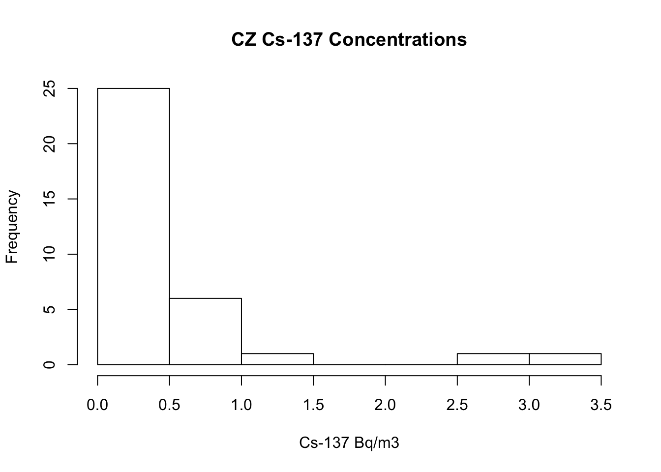
hist(air$Cs.137..Bq.m3.[air$PAYS == "AU"], main = "AU Cs-137 Concentrations",
xlab = "Cs-137 Bq/m3") #normality violated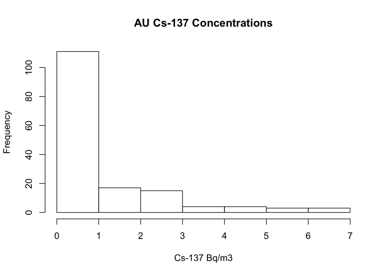 I went on to conduct the Mann-Whitney U-test. Below I stated the null and alternative hypotheses:
Ho: The distribution of mean concentrations for Cs-137 between Czechoslovakia and Austria are the same.
Ha: The distribution of mean concentrations for Cs-137 between Czechoslovakia and Austria differ significantly.
CZ.AU.Cs137 <- air %>% select(PAYS, Ville, Cs.137..Bq.m3.) %>%
    filter(PAYS %in% c("CZ", "AU"))
wilcox.test(CZ.AU.Cs137$Cs.137..Bq.m3. ~ CZ.AU.Cs137$PAYS)
##
## Wilcoxon rank sum test with continuity correction
##
## data: CZ.AU.Cs137$Cs.137..Bq.m3. by CZ.AU.Cs137$PAYS
## W = 3623, p-value = 0.001104
## alternative hypothesis: true location shift is not equal to 0The results from the test came back significant. The null hypothesis that the mean concentrations for Cs-137 were equal between the two countries could be rejected (W = 3623, n = (34,157), p = 0.0011). It appears Austria had higher concentrations of recorded Cs-137 compared to Czechoslovakia.
CONCLUSIONS
The statistical analysis supports the research concerning how radioactive fallout spread throughout Europe following the Chernobyl disaster. Just because a particular country was closer geographically did not necessarily mean higher concentrations of Cs-137 were recorded. Austria was shown to have significantly higher concentrations of Cs-137 when compared to its neighbor Czechoslovakia. In the future it could be interesting to explore ggplot2 further to code a map of Europe with countries shaded based on their mean concentrations of Cs-137. This could further help with visualization of Cs-137 concentrations across Europe as well as provoke more ideas for additional statistical analysis.
SOURCES
Petryna, A. (2013). Life exposed: biological citizens after Chernobyl. Princeton University Press.
Bossew, P., Ditto, M., Falkner, T., Henrich, E., Kienzl, K., & Rappelsberger, U. (2001). Contamination of Austrian soil with caesium-137. Journal of environmental radioactivity, 55(2), 187–194. https://doi.org/10.1016/s0265-931x(00)00192-2
Zablotska L. B. (2016). 30 years After the Chernobyl Nuclear Accident: Time for Reflection and Re-evaluation of Current Disaster Preparedness Plans. Journal of urban health : bulletin of the New York Academy of Medicine, 93(3), 407–413. https://doi.org/10.1007/s11524-016-0053-x
Avery, S. V. (1996). Fate of caesium in the environment: distribution between the abiotic and biotic components of aquatic and terrestrial ecosystems. Journal of Environmental Radioactivity, 30(2), 139-171.
DATA
glimpse(air)## Rows: 1,531
## Columns: 11
## $ PAYS <fct> SE, SE, SE, SE, SE, SE, SE, SE, SE, SE, SE, SE, SE, S…
## $ Code <int> 1, 1, 1, 1, 1, 1, 1, 1, 1, 1, 1, 1, 1, 1, 1, 1, 1, 1,…
## $ Ville <fct> RISOE, RISOE, RISOE, RISOE, RISOE, RISOE, RISOE, RISO…
## $ X <dbl> 12.07, 12.07, 12.07, 12.07, 12.07, 12.07, 12.07, 12.0…
## $ Y <dbl> 55.7, 55.7, 55.7, 55.7, 55.7, 55.7, 55.7, 55.7, 55.7,…
## $ Date <fct> 86/04/27, 86/04/28, 86/04/29, 86/04/29, 86/04/30, 86/…
## $ End.of.sampling <fct> 24:00:00, 24:00:00, 12:00, 24:00:00, 24:00:00, 24:00:…
## $ Duration.h.min. <dbl> 24, 24, 12, 12, 24, 24, 24, 24, 12, 12, 12, 12, 12, 1…
## $ I.131..Bq.m3. <dbl> 1.000000, 0.004600, 0.014700, 0.000610, 0.000750, 0.0…
## $ Cs.134..Bq.m3. <dbl> 0.000000, 0.000540, 0.004300, 0.000000, 0.000100, 0.0…
## $ Cs.137..Bq.m3. <dbl> 0.240000, 0.000980, 0.007400, 0.000090, 0.000280, 0.0…