January 1, 0001
Modeling Covid-19
library(tidyverse)
library(lmtest)
library(sandwich)
covid <- read.csv("//Users/bitoFLO/Desktop/Website/content/1_county_level_confirmed_cases(1).csv",
    header = T, na.strings = c("", "NA"))
covid <- covid %>% na.omit()
The dataset I found collected by John Hopkins University (Johns Hopkins University’s COVID-19 tracking project) contains data relevant to the novel coronavirus pertaining to the United States. The data concerns confirmed cases, deaths, confirmed cases per 100,000 people, and deaths per 100,000 people for various counties in each state as of April 21st, 2020. The total population for each county is also recorded and these counties are further classified into one of six urbanization categories varying from ‘non-core’ to ‘large central metropolitan’. There are 2812 observations, although only 2756 had values for all variables listed, so 56 observations were omitted since they contained NA’s for at least one of the variables of interest. An important consideration is that this dataset reflects the availability of COVID-19 tests rather than true infection rates. Likewise, this data reveals the results of the tests for those that were able to be tested. Certain counties will have more access to these tests while others will have limited access, so this should also be taken into consideration.
MANOVA
mancovid <- manova(cbind(total_population, deaths, confirmed,
    deaths_per_100000, confirmed_per_100000) ~ NCHS_urbanization,
    data = covid)
summary(mancovid)
## Df Pillai approx F num Df den Df Pr(>F)
## NCHS_urbanization 5 0.44268 53.424 25 13750 < 2.2e-16 ***
## Residuals 2750
## ---
## Signif. codes: 0 '***' 0.001 '**' 0.01 '*' 0.05 '.' 0.1 ' ' 1summary.aov(mancovid)## Response total_population :
## Df Sum Sq Mean Sq F value Pr(>F)
## NCHS_urbanization 5 1.5145e+14 3.0291e+13 346.17 < 2.2e-16 ***
## Residuals 2750 2.4063e+14 8.7503e+10
## ---
## Signif. codes: 0 '***' 0.001 '**' 0.01 '*' 0.05 '.' 0.1 ' ' 1
##
## Response deaths :
## Df Sum Sq Mean Sq F value Pr(>F)
## NCHS_urbanization 5 8382574 1676515 21.485 < 2.2e-16 ***
## Residuals 2750 214587288 78032
## ---
## Signif. codes: 0 '***' 0.001 '**' 0.01 '*' 0.05 '.' 0.1 ' ' 1
##
## Response confirmed :
## Df Sum Sq Mean Sq F value Pr(>F)
## NCHS_urbanization 5 1.8279e+09 365574161 43.69 < 2.2e-16 ***
## Residuals 2750 2.3010e+10 8367400
## ---
## Signif. codes: 0 '***' 0.001 '**' 0.01 '*' 0.05 '.' 0.1 ' ' 1
##
## Response deaths_per_100000 :
## Df Sum Sq Mean Sq F value Pr(>F)
## NCHS_urbanization 5 14337 2867.36 19.987 < 2.2e-16 ***
## Residuals 2750 394522 143.46
## ---
## Signif. codes: 0 '***' 0.001 '**' 0.01 '*' 0.05 '.' 0.1 ' ' 1
##
## Response confirmed_per_100000 :
## Df Sum Sq Mean Sq F value Pr(>F)
## NCHS_urbanization 5 6117946 1223589 27.949 < 2.2e-16 ***
## Residuals 2750 120393078 43779
## ---
## Signif. codes: 0 '***' 0.001 '**' 0.01 '*' 0.05 '.' 0.1 ' ' 1pairwise.t.test(covid$total_population, covid$NCHS_urbanization,
p.adj = "none")##
## Pairwise comparisons using t tests with pooled SD
##
## data: covid$total_population and covid$NCHS_urbanization
##
## Large central metro Large fringe metro Medium metro
## Large fringe metro < 2e-16 - -
## Medium metro < 2e-16 0.11735 -
## Micropolitan < 2e-16 < 2e-16 8.1e-13
## Non-core < 2e-16 < 2e-16 < 2e-16
## Small metro < 2e-16 1.1e-09 5.5e-06
## Micropolitan Non-core
## Large fringe metro - -
## Medium metro - -
## Micropolitan - -
## Non-core 0.07462 -
## Small metro 0.04496 0.00028
##
## P value adjustment method: nonepairwise.t.test(covid$deaths, covid$NCHS_urbanization, p.adj = "none")##
## Pairwise comparisons using t tests with pooled SD
##
## data: covid$deaths and covid$NCHS_urbanization
##
## Large central metro Large fringe metro Medium metro
## Large fringe metro <2e-16 - -
## Medium metro <2e-16 0.280 -
## Micropolitan <2e-16 0.090 0.628
## Non-core <2e-16 0.059 0.564
## Small metro <2e-16 0.158 0.731
## Micropolitan Non-core
## Large fringe metro - -
## Medium metro - -
## Micropolitan - -
## Non-core 0.948 -
## Small metro 0.925 0.877
##
## P value adjustment method: nonepairwise.t.test(covid$confirmed, covid$NCHS_urbanization, p.adj = "none")##
## Pairwise comparisons using t tests with pooled SD
##
## data: covid$confirmed and covid$NCHS_urbanization
##
## Large central metro Large fringe metro Medium metro
## Large fringe metro < 2e-16 - -
## Medium metro < 2e-16 0.01166 -
## Micropolitan < 2e-16 0.00011 0.29781
## Non-core < 2e-16 1.5e-05 0.20283
## Small metro < 2e-16 0.00151 0.49827
## Micropolitan Non-core
## Large fringe metro - -
## Medium metro - -
## Micropolitan - -
## Non-core 0.85949 -
## Small metro 0.78683 0.66170
##
## P value adjustment method: nonepairwise.t.test(covid$deaths_per_100000, covid$NCHS_urbanization,
p.adj = "none")##
## Pairwise comparisons using t tests with pooled SD
##
## data: covid$deaths_per_100000 and covid$NCHS_urbanization
##
## Large central metro Large fringe metro Medium metro
## Large fringe metro 3.6e-06 - -
## Medium metro 3.6e-11 0.00024 -
## Micropolitan 1.5e-14 5.3e-09 0.08417
## Non-core 5.0e-15 3.0e-10 0.06341
## Small metro 1.0e-11 6.2e-05 0.70857
## Micropolitan Non-core
## Large fringe metro - -
## Medium metro - -
## Micropolitan - -
## Non-core 0.99009 -
## Small metro 0.19826 0.16841
##
## P value adjustment method: nonepairwise.t.test(covid$confirmed_per_100000, covid$NCHS_urbanization,
p.adj = "none")##
## Pairwise comparisons using t tests with pooled SD
##
## data: covid$confirmed_per_100000 and covid$NCHS_urbanization
##
## Large central metro Large fringe metro Medium metro
## Large fringe metro 1.0e-04 - -
## Medium metro 3.2e-12 1.4e-08 -
## Micropolitan 1.8e-14 2.9e-13 0.3439
## Non-core < 2e-16 < 2e-16 0.0419
## Small metro 2.3e-11 2.8e-07 0.6292
## Micropolitan Non-core
## Large fringe metro - -
## Medium metro - -
## Micropolitan - -
## Non-core 0.2268 -
## Small metro 0.1407 0.0098
##
## P value adjustment method: none# 81 tests performed total
1 - 0.95^81## [1] 0.98431040.9843104/81## [1] 0.01215198The first test performed was the MANOVA to determine if any of the response variables (total_populations, deaths, confirmed, confirmed_per_100000, and deaths_per_100000) differed based on the categorical variable ‘NCHS_urbanization’. It tested whether the means of the groups were equal. The MANOVA came back significant indicating at least one of the urbanization categories differed for one of the response variables, Pillai trace = .443, pseudo F(5,13750) = 53.424, p < .0001.
Univariate ANOVAs were then conducted for each response variable: total_populations, deaths, confirmed, confirmed_per_100000, and deaths_per_100000 to find which ones showed a mean difference across the groups. All responses were found to be significant using the bonferroni method to control for the type-I error; F = 346.17 with p < .0001, F = 21.485 with p < .0001, F = 43.69 with p < .0001, F = 19.987 with p < .0001, and F = 27.949 with p < .0001 respectively. The post-hoc t-tests tested to see which urbanization categories differed among the five response variables. The large central metro was shown to differ from the five other groups among every response variable when using the bonferroni correction of .01215. It was interesting to find that among the six urbanization categories, only the large central metro differed from the others in number of deaths from COVID-19. The large fringe metro was also showed significant differences between the other categories when variables such as confirmed cases, deaths per 100,000, and confirmed cases per 100,000 were concerned. Another interesting significant difference in means is between ‘non-core’ and ‘small metro’ for the response confirmed cases per 100,000, even though they are not significantly different for confirmed cases.
All in all, 81 tests were conducted and the probability of making at least one type-I error is extremely high at 98%. This is why an adjusted bonferroni significance level of .012 was used in order to keep type-I error rate at 5%. Most likely the assumption for random sampling and independent observations was not met because of testing being largely due to the amount of resources available for each particular county. When extreme outliers are concerned among the response variables, it is apparent the large central metro meets this criterion for every single post-hot t-test. However, the great number of observations may have still resulted in multivariate normallity.
Randomization Test (PERMANOVA)
library(vegan)
coviddists <- covid %>% select(confirmed_per_100000, total_population) %>%
    dist()
adoniscovid <- adonis(coviddists ~ NCHS_urbanization, data = covid)
adoniscovid
##
## Call:
## adonis(formula = coviddists ~ NCHS_urbanization, data = covid)
##
## Permutation: free
## Number of permutations: 999
##
## Terms added sequentially (first to last)
##
## Df SumsOfSqs MeanSqs F.Model R2 Pr(>F)
## NCHS_urbanization 5 1.5145e+14 3.0291e+13 346.17 0.38628 0.001 ***
## Residuals 2750 2.4063e+14 8.7503e+10 0.61372
## Total 2755 3.9209e+14 1.00000
## ---
## Signif. codes: 0 '***' 0.001 '**' 0.01 '*' 0.05 '.' 0.1 ' ' 1qplot(adoniscovid$f.perms) + geom_vline(xintercept = 346.17,
color = "red") + scale_x_log10() + ggtitle("Plotted Null Distribution and Test Statistic (Logarithmic Scale)") +
xlab("F-stat permutations") + theme(plot.title = element_text(hjust = 0.5))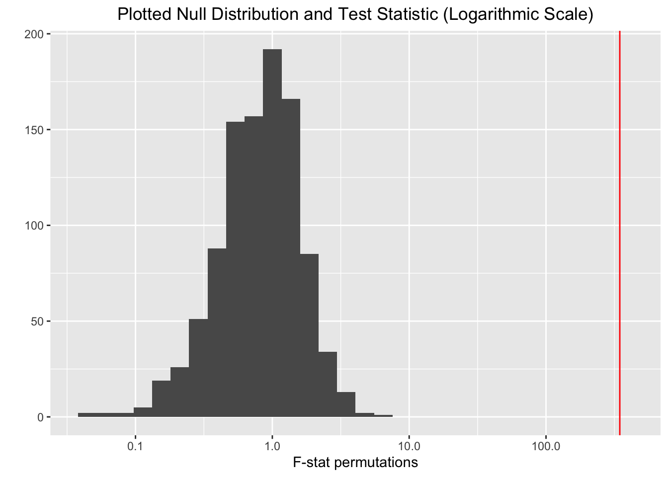
The PERMANOVA was conducted because of the ease of use for conducting an effective randomization test via the ‘vegan’ package. Using the ‘adonis’ function only two lines of code were needed to perform a randomization test with 999 permutations. Another reason the PERMANOVA was ideal was the nice departure from the MANOVA it offered since the endless assumptions one must meet (that are often violated) for a MANOVA are non-existent in the PERMANOVA.
H0: The multivariate means of the distances between total population and confirmed cases per 100,000 for each of the urbanization categories are equal.
HA: At least one of the urbanization categories differs in the multivariate means for the distances between total population and confirmed cases per 100,000.
There is shown to be a significant difference so one can reject the null hypothesis. The multivariate means of the distances for at least one of the urbanization categories is not equal (F = 346.17, p < .001). It is interesting to see this result especially when using the ‘confirmed per 100,000’ variable that puts the distances between this variable and the total populations of each county on a more even playing field.
Linear Regression Model
covid$total_population_c <- covid$total_population - mean(covid$total_population,
    na.rm = TRUE)
covid$NCHS_urbanization <- relevel(covid$NCHS_urbanization, ref = "Medium metro")
linear <- lm(confirmed ~ total_population_c * NCHS_urbanization,
    data = covid)
summary(linear)
##
## Call:
## lm(formula = confirmed ~ total_population_c * NCHS_urbanization,
## data = covid)
##
## Residuals:
## Min 1Q Median 3Q Max
## -43178 -26 -6 11 94244
##
## Coefficients:
## Estimate Std. Error
## (Intercept) 1.263e+02 1.298e+02
## total_population_c 1.633e-03 6.086e-04
## NCHS_urbanizationLarge central metro -3.524e+03 4.025e+02
## NCHS_urbanizationLarge fringe metro 9.898e+01 1.830e+02
## NCHS_urbanizationMicropolitan -2.123e+01 3.084e+02
## NCHS_urbanizationNon-core -2.401e+01 6.532e+02
## NCHS_urbanizationSmall metro 2.372e+00 1.916e+02
## total_population_c:NCHS_urbanizationLarge central metro 4.418e-03 6.318e-04
## total_population_c:NCHS_urbanizationLarge fringe metro 3.741e-03 7.302e-04
## total_population_c:NCHS_urbanizationMicropolitan -7.185e-04 3.698e-03
## total_population_c:NCHS_urbanizationNon-core -7.312e-04 6.437e-03
## total_population_c:NCHS_urbanizationSmall metro -4.862e-04 2.079e-03
## t value Pr(>|t|)
## (Intercept) 0.973 0.33048
## total_population_c 2.683 0.00733 **
## NCHS_urbanizationLarge central metro -8.756 < 2e-16 ***
## NCHS_urbanizationLarge fringe metro 0.541 0.58867
## NCHS_urbanizationMicropolitan -0.069 0.94512
## NCHS_urbanizationNon-core -0.037 0.97069
## NCHS_urbanizationSmall metro 0.012 0.99012
## total_population_c:NCHS_urbanizationLarge central metro 6.992 3.38e-12 ***
## total_population_c:NCHS_urbanizationLarge fringe metro 5.123 3.22e-07 ***
## total_population_c:NCHS_urbanizationMicropolitan -0.194 0.84597
## total_population_c:NCHS_urbanizationNon-core -0.114 0.90957
## total_population_c:NCHS_urbanizationSmall metro -0.234 0.81511
## ---
## Signif. codes: 0 '***' 0.001 '**' 0.01 '*' 0.05 '.' 0.1 ' ' 1
##
## Residual standard error: 2340 on 2744 degrees of freedom
## Multiple R-squared: 0.3948, Adjusted R-squared: 0.3924
## F-statistic: 162.8 on 11 and 2744 DF, p-value: < 2.2e-16covid %>% ggplot(aes(total_population_c, confirmed)) + geom_point(aes(color = NCHS_urbanization)) +
geom_smooth(method = "lm", se = F)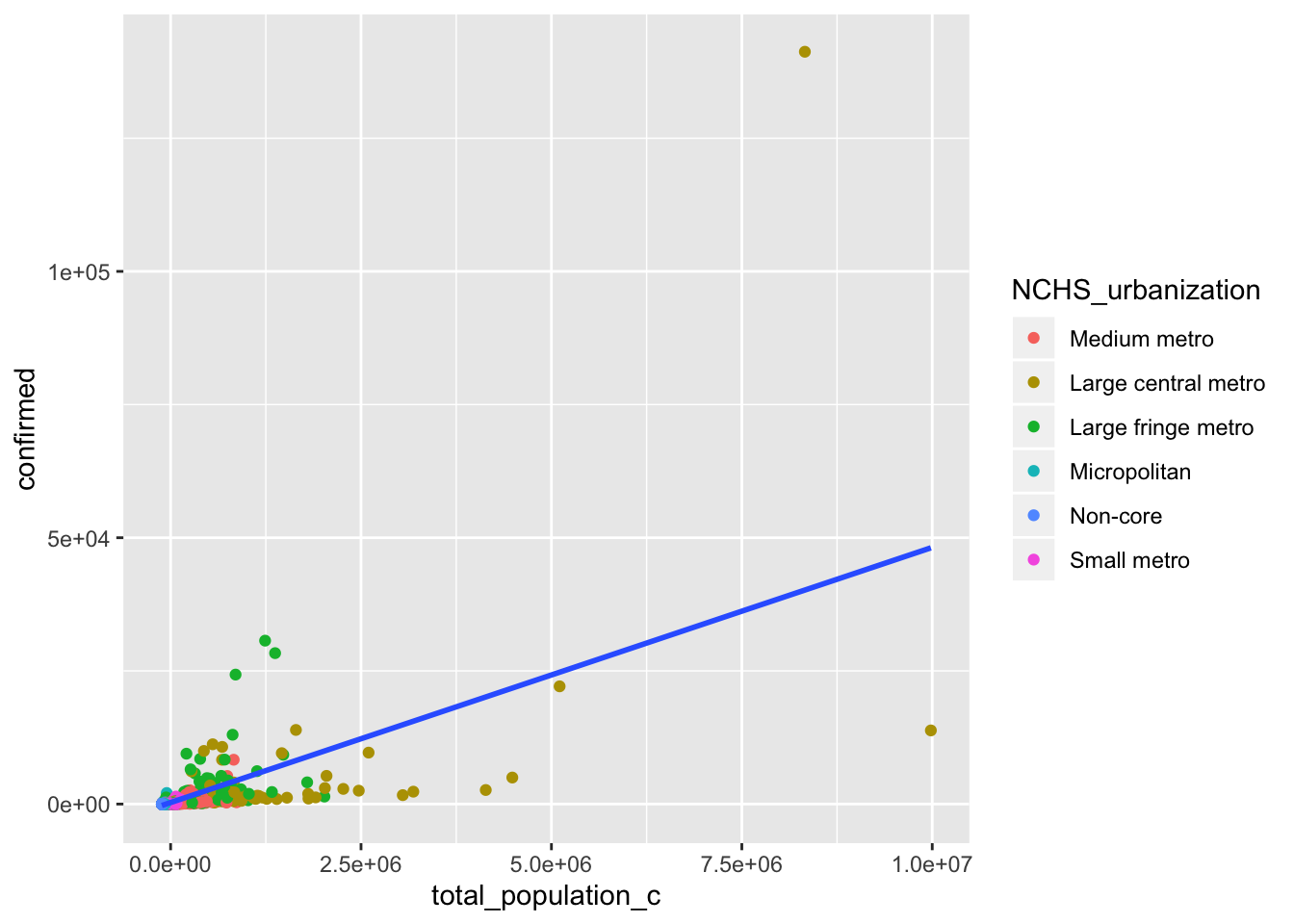
resids <- lm(confirmed ~ total_population_c, data = covid)$residuals
fitted <- lm(confirmed ~ total_population_c, data = covid)$fitted.values
shapiro.test(resids)
##
## Shapiro-Wilk normality test
##
## data: resids
## W = 0.13509, p-value < 2.2e-16ggplot() + geom_point(aes(fitted, resids)) + geom_hline(yintercept = 0,
color = "green")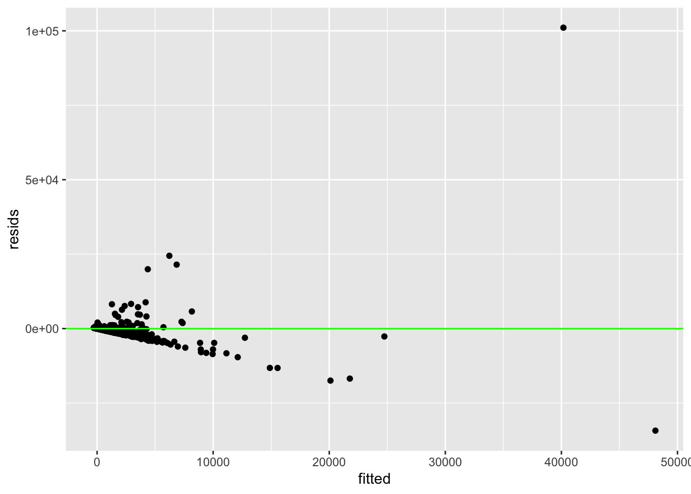
ggplot(linear, aes(total_population_c, confirmed)) + geom_point() +
    geom_smooth(method = lm, se = F)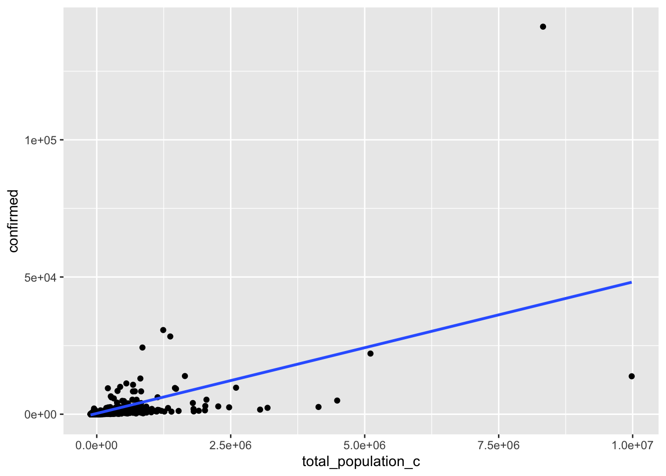
bptest(linear)##
## studentized Breusch-Pagan test
##
## data: linear
## BP = 1187.5, df = 11, p-value < 2.2e-16coeftest(linear, vcov = vcovHC(linear))##
## t test of coefficients:
##
## Estimate Std. Error
## (Intercept) 1.2631e+02 1.1992e+01
## total_population_c 1.6331e-03 4.4848e-04
## NCHS_urbanizationLarge central metro -3.5245e+03 5.8887e+03
## NCHS_urbanizationLarge fringe metro 9.8979e+01 6.4297e+01
## NCHS_urbanizationMicropolitan -2.1229e+01 2.2655e+01
## NCHS_urbanizationNon-core -2.4008e+01 2.7340e+01
## NCHS_urbanizationSmall metro 2.3722e+00 1.7706e+01
## total_population_c:NCHS_urbanizationLarge central metro 4.4177e-03 5.6947e-03
## total_population_c:NCHS_urbanizationLarge fringe metro 3.7406e-03 1.5556e-03
## total_population_c:NCHS_urbanizationMicropolitan -7.1850e-04 5.0310e-04
## total_population_c:NCHS_urbanizationNon-core -7.3120e-04 5.0938e-04
## total_population_c:NCHS_urbanizationSmall metro -4.8619e-04 4.8015e-04
## t value Pr(>|t|)
## (Intercept) 10.5328 < 2.2e-16 ***
## total_population_c 3.6413 0.0002762 ***
## NCHS_urbanizationLarge central metro -0.5985 0.5495448
## NCHS_urbanizationLarge fringe metro 1.5394 0.1238220
## NCHS_urbanizationMicropolitan -0.9370 0.3488218
## NCHS_urbanizationNon-core -0.8781 0.3799538
## NCHS_urbanizationSmall metro 0.1340 0.8934291
## total_population_c:NCHS_urbanizationLarge central metro 0.7758 0.4379583
## total_population_c:NCHS_urbanizationLarge fringe metro 2.4047 0.0162527 *
## total_population_c:NCHS_urbanizationMicropolitan -1.4281 0.1533641
## total_population_c:NCHS_urbanizationNon-core -1.4355 0.1512646
## total_population_c:NCHS_urbanizationSmall metro -1.0126 0.3113492
## ---
## Signif. codes: 0 '***' 0.001 '**' 0.01 '*' 0.05 '.' 0.1 ' ' 1(sum((covid$confirmed - mean(covid$confirmed))^2) - sum(linear$residuals^2))/sum((covid$confirmed -
mean(covid$confirmed))^2)## [1] 0.3948395The intercept of regressing ‘confirmed’ on the predictors ‘NCHS_urbanization’ and ‘total_population_c’ tell how much each observation differed from the mean value for ‘total_population’. The intercept summarizes the value for ‘confirmed’ (126.3) when the reference group ‘medium metro’ has a ‘total_population’ equal to the mean. The coefficient ‘total_population_c’ (.001633) shows confirmed cases increase as the total population increases. The coefficient ‘NCHS_urbanization large fringe metro’ and ‘NCHS_urbanization small metro’ show these two urbanization categories on average will have increased confirmed cases from the reference group opposed to the other three categories The interactions shows if the effect of ‘total_population_c’ differ on the level of urbanization category. ‘Total_population_c:NCHS_urbanization large central metro’ and ‘total_population_c:NCHS_urbanization large fringe metro’ were the two interactions that were both positive and significant.
After conducting a Shapiro-Wilk normality test, it was apparent this model is not normally distributed since the null hypothesis can be rejected (p<.05). When testing for linearity a scatterplot was used and after eyeballing the pattern of the points and where they were clustered together this assumption also appears to be violated. Homoscedasticity does not seem to be met as the points fan outwards, and the Breuch-Pagan test proves this (p<.05), therefore the null hypothesis for homoscedasticity can also be rejected.
Due to heteroskedasticity, robust standard errors were appropriate to incorporate into the model. When these were incorporated the ‘large central metro’ was no longer significant along with the interactions ‘total_population_c:NCHS_urbanization large central metro’ and ‘total_population_c:NCHS_urbanization large fringe metro’. ‘Total_population_c’ remained significant as the standard error and p-value both decreased (p<.001). ‘Total_population_c:NCHS_urbanization large fringe metro’ also remained significant, but standard error increased along with the p-value.
After calculating the R-squared value it showed that 0.395 of the variation in confirmed cases could be explained by the model including the two predictors, urbanization category and total population of the county.
Bootstrapped Standard Errors
linear <- lm(confirmed ~ total_population_c * NCHS_urbanization,
    data = covid)
resids <- lm(confirmed ~ total_population_c, data = covid)$residuals
fitted <- lm(confirmed ~ total_population_c, data = covid)$fitted.values
resid_resample <- replicate(5000, {
    new_resids <- sample(resids, replace = TRUE)
    covid$new_y <- fitted + new_resids
    linearresid <- lm(new_y ~ total_population_c * NCHS_urbanization,
        data = covid)
    coef(linearresid)
})
resid_resample %>% t %>% as.data.frame %>% summarize_all(sd)
## (Intercept) total_population_c NCHS_urbanizationLarge central metro
## 1 133.7631 0.0006240891 398.1188
## NCHS_urbanizationLarge fringe metro NCHS_urbanizationMicropolitan
## 1 186.3176 312.2634
## NCHS_urbanizationNon-core NCHS_urbanizationSmall metro
## 1 665.2336 195.8255
## total_population_c:NCHS_urbanizationLarge central metro
## 1 0.0006428125
## total_population_c:NCHS_urbanizationLarge fringe metro
## 1 0.0007566298
## total_population_c:NCHS_urbanizationMicropolitan
## 1 0.003740542
## total_population_c:NCHS_urbanizationNon-core
## 1 0.006573827
## total_population_c:NCHS_urbanizationSmall metro
## 1 0.002094365coeftest(linear)[, 1:2]## Estimate
## (Intercept) 1.263098e+02
## total_population_c 1.633057e-03
## NCHS_urbanizationLarge central metro -3.524484e+03
## NCHS_urbanizationLarge fringe metro 9.897925e+01
## NCHS_urbanizationMicropolitan -2.122869e+01
## NCHS_urbanizationNon-core -2.400795e+01
## NCHS_urbanizationSmall metro 2.372174e+00
## total_population_c:NCHS_urbanizationLarge central metro 4.417745e-03
## total_population_c:NCHS_urbanizationLarge fringe metro 3.740637e-03
## total_population_c:NCHS_urbanizationMicropolitan -7.185011e-04
## total_population_c:NCHS_urbanizationNon-core -7.312046e-04
## total_population_c:NCHS_urbanizationSmall metro -4.861918e-04
## Std. Error
## (Intercept) 1.297712e+02
## total_population_c 6.085933e-04
## NCHS_urbanizationLarge central metro 4.025018e+02
## NCHS_urbanizationLarge fringe metro 1.830151e+02
## NCHS_urbanizationMicropolitan 3.083709e+02
## NCHS_urbanizationNon-core 6.532466e+02
## NCHS_urbanizationSmall metro 1.916158e+02
## total_population_c:NCHS_urbanizationLarge central metro 6.318053e-04
## total_population_c:NCHS_urbanizationLarge fringe metro 7.301615e-04
## total_population_c:NCHS_urbanizationMicropolitan 3.698230e-03
## total_population_c:NCHS_urbanizationNon-core 6.437436e-03
## total_population_c:NCHS_urbanizationSmall metro 2.079009e-03coeftest(linear, vcovHC(linear))[, 1:2]## Estimate
## (Intercept) 1.263098e+02
## total_population_c 1.633057e-03
## NCHS_urbanizationLarge central metro -3.524484e+03
## NCHS_urbanizationLarge fringe metro 9.897925e+01
## NCHS_urbanizationMicropolitan -2.122869e+01
## NCHS_urbanizationNon-core -2.400795e+01
## NCHS_urbanizationSmall metro 2.372174e+00
## total_population_c:NCHS_urbanizationLarge central metro 4.417745e-03
## total_population_c:NCHS_urbanizationLarge fringe metro 3.740637e-03
## total_population_c:NCHS_urbanizationMicropolitan -7.185011e-04
## total_population_c:NCHS_urbanizationNon-core -7.312046e-04
## total_population_c:NCHS_urbanizationSmall metro -4.861918e-04
## Std. Error
## (Intercept) 1.199201e+01
## total_population_c 4.484759e-04
## NCHS_urbanizationLarge central metro 5.888700e+03
## NCHS_urbanizationLarge fringe metro 6.429730e+01
## NCHS_urbanizationMicropolitan 2.265512e+01
## NCHS_urbanizationNon-core 2.734007e+01
## NCHS_urbanizationSmall metro 1.770559e+01
## total_population_c:NCHS_urbanizationLarge central metro 5.694742e-03
## total_population_c:NCHS_urbanizationLarge fringe metro 1.555569e-03
## total_population_c:NCHS_urbanizationMicropolitan 5.031011e-04
## total_population_c:NCHS_urbanizationNon-core 5.093802e-04
## total_population_c:NCHS_urbanizationSmall metro 4.801506e-04After bootstrapping the residuals of the linear model, the coefficient estimates remained the same as those in the original model and the model without the robust standard error bars. The changes were found in the standard errors as well as the significance level. The robust standard errors now offer a more conservative consensus for what coefficients are significant for the model. With the outliers in the dataset, it is best practice to go off the model including the robust standard errors. The bootstrapped residuals compare most closely to the standard errors of the initial linear model without robust standard errors. The standard errors of these bootstrapped residuals are slightly greater than the original standard errors
Logistic Regression
library(plotROC)
covid <- covid %>% mutate(y = ifelse(NCHS_urbanization == "Large central metro",
    1, 0))
logistic <- glm(y ~ confirmed_per_100000 + deaths_per_100000 +
    total_population, data = covid, family = binomial(link = "logit"))
coeftest(logistic)
##
## z test of coefficients:
##
## Estimate Std. Error z value Pr(>|z|)
## (Intercept) -5.7838e+00 3.0610e-01 -18.8947 <2e-16 ***
## confirmed_per_100000 -5.3832e-04 1.0177e-03 -0.5289 0.5968
## deaths_per_100000 1.5897e-02 1.8775e-02 0.8467 0.3972
## total_population 5.4541e-06 4.4594e-07 12.2305 <2e-16 ***
## ---
## Signif. codes: 0 '***' 0.001 '**' 0.01 '*' 0.05 '.' 0.1 ' ' 1exp(coef(logistic))## (Intercept) confirmed_per_100000 deaths_per_100000
## 0.003077133 0.999461827 1.016023977
## total_population
## 1.000005454probs <- predict(logistic, type = "response")
table(predict = as.numeric(probs > 0.5), truth = covid$y) %>%
addmargins #reported confusion matrix for 'logistic'## truth
## predict 0 1 Sum
## 0 2683 37 2720
## 1 9 27 36
## Sum 2692 64 2756class_diag <- function(probs, truth) {
if (is.numeric(truth) == FALSE & is.logical(truth) == FALSE)
truth <- as.numeric(truth) - 1
tab <- table(factor(probs > 0.5, levels = c("FALSE", "TRUE")),
truth)
prediction <- ifelse(probs > 0.5, 1, 0)
acc = mean(truth == prediction)
sens = mean(prediction[truth == 1] == 1)
spec = mean(prediction[truth == 0] == 0)
ppv = mean(truth[prediction == 1] == 1)
ord <- order(probs, decreasing = TRUE)
probs <- probs[ord]
truth <- truth[ord]
TPR = cumsum(truth)/max(1, sum(truth))
FPR = cumsum(!truth)/max(1, sum(!truth))
dup <- c(probs[-1] >= probs[-length(probs)], FALSE)
TPR <- c(0, TPR[!dup], 1)
FPR <- c(0, FPR[!dup], 1)
n <- length(TPR)
auc <- sum(((TPR[-1] + TPR[-n])/2) * (FPR[-1] - FPR[-n]))
data.frame(acc, sens, spec, ppv, auc)
}
problogistic <- predict(logistic, type = "response")
class_diag(problogistic, covid$y)## acc sens spec ppv auc
## 1 0.9833091 0.421875 0.9966568 0.75 0.9860118logit <- function(p) log(odds(p))
covid$logit <- predict(logistic)
covid$y <- factor(covid$y, levels = c("1", "0"))
covid %>% ggplot() + geom_density(aes(logit, color = y, fill = y),
alpha = 0.4) + theme(legend.position = c(0.85, 0.85)) + geom_vline(xintercept = 0) +
xlab("predictor (logit)")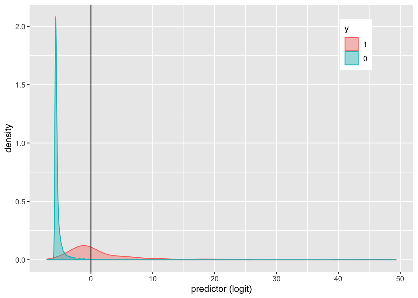
ROClogistic <- ggplot(logistic) + geom_roc(aes(d = y, m = confirmed_per_100000 +
    deaths_per_100000 + total_population), n.cuts = 0) + geom_segment(aes(x = 0,
    xend = 1, y = 0, yend = 1), lty = 2)
ROClogistic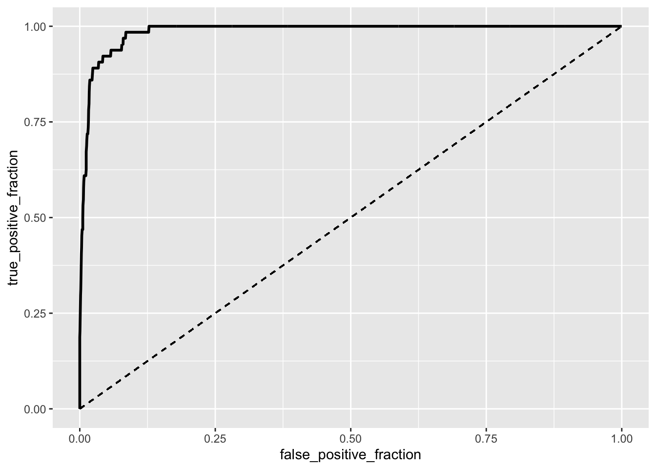
calc_auc(ROClogistic)## PANEL group AUC
## 1 1 -1 0.986244k = 10
data <- covid[sample(nrow(covid)), ]
folds <- cut(seq(1:nrow(covid)), breaks = k, labels = F)
diags <- NULL
for (i in 1:k) {
train <- data[folds != i, ]
test <- data[folds == i, ]
truth <- test$y
logistic <- glm(y ~ confirmed_per_100000 + deaths_per_100000 +
total_population, data = covid, family = binomial(link = "logit"))
probs <- predict(logistic, newdata = test, type = "response")
diags <- rbind(diags, class_diag(probs, truth))
}
summarize_all(diags, mean)## acc sens spec ppv auc
## 1 0.9833057 0.996639 0.412619 0.9864042 0.985028Mutate was first used to create a new binary variable ‘y’ in the dataset that output 1 if the urbanization area was a large central metropolitan and a 0 if it was not (any of the other 5 urbanization categories). I thought this was interesting because it allows viewing of how the “big cities” compared to each other as well as the other urbanization categories. “Y” was predicted from three explanatory variables: ‘confirmed_per_100000’, ‘deaths_per_100000’, and ‘total_population’ and then exponentiated to obtain the odds for each coefficient opposed to making sense of the log odds obtained from the logistic regression. The intercept coefficient shows the odds of a county being from a large central metropolitan when the confirmed cases per 100,000, deaths per 100,000, and total population are all equal to 0 (odds = .0031). It makes sense the odds are incredibly low for this. When controlling for ‘deaths_per_100000’ and ‘total_population’, for every additional unit in ‘confirmed_per_100000’ the odds of a county being a large central metropolitan increase by almost 1 (.9995) but was not significant (p > .05). Likewise, when controlling for ‘confirmed_per_100000’ and ‘total_population’, for every additional unit in ‘deaths_per_100000’ the odds of a county being a large central metropolitan increase by over 1 (1.016) yet is still not significant (p > .05). Lastly, when controlling for ‘deaths_per_100000’ and ‘confirmed_per_100000’, for every additional unit in ‘total_population’ the odds of a county being a large central metropolitan increase by 1 and is significant (p < .001). This intuitively makes sense as population is the greatest indicator where a county stands when the urbanization category is concerned.
After making the confusion matrix the accuracy, sensitivity, specificity, and precision could be calculated. However, the ‘class_diag’ function written by Dr. Woodward was used to easily get these measures instead. The proportion of observations that were correctly classified (accuracy) was .983. A proportion of .422 of the urbanization category ‘large central metro’ were classified correctly (the true positive rate) and .997 of observations that did not fall in the ‘large central metro’ category were classified correctly (the true negative rate). The precision stood at a proportion of .75 observations classified as ‘large central metro’ that actually were. Overall it seems the model does well at predicting an observation that falls in the urbanization category ‘large central metro’ from the three explanatory variables.
The significant output from the GLM foreshadows that this model may be a good predictor for the binary variable: ‘Large central metro’ (1) and ‘Not large central metro’ (0). The ROC curve works as a visual representation for how well the model is able to differentiate between these two classifications by using the measures of sensitivity and septicity. The ROC curve is great since it stays away from the dashed line as it shoots upwards almost to 1 and then right directly following the tick on the y-axis at 1. The curve illustrates how strong the AUC (the area under the curve) will be and after calculating AUC with the plotROC package, it can be seen the AUC is great at .986. This value for AUC summarizes what the ROC curve shows, but in just one value. Both tell us our model is indeed a great predictor for the binary variable when given the predictors.
A tenfold cross validation was conducted to see how the model would predict new data based on the current data. After viewing the results, it is apparent the model is still a great predictor of the binary variable with an AUC = .986. The out of sample accuracy, sensitivity, and recall were .983, .997, and .442 respectively. It was interesting to see that the values for sensitivity and recall essentially switched places between the model estimates and the out-of-sample averages.
Lasso
library(glmnet)
y <- as.matrix(covid$y)
x <- covid %>% select(total_population, confirmed, confirmed_per_100000,
    deaths, deaths_per_100000) %>% mutate_all(scale) %>% as.matrix
cv <- cv.glmnet(x, y, family = "binomial")
lasso <- glmnet(x, y, family = "binomial", lambda = cv$lambda.1se)
coef(lasso)
## 6 x 1 sparse Matrix of class "dgCMatrix"
## s0
## (Intercept) -4.0953611
## total_population 0.8901898
## confirmed .
## confirmed_per_100000 .
## deaths .
## deaths_per_100000 .k = 10
data <- covid %>% sample_frac
fold <- ntile(1:nrow(data), n = 10)
diags <- NULL
for (i in 1:k) {
train <- data[folds != i, ]
test <- data[folds == i, ]
truth <- test$y
lassofit <- glm(y ~ total_population, data = train, family = "binomial")
probs <- predict(lassofit, newdata = test, type = "response")
diags <- rbind(diags, class_diag(probs, truth))
}
diags %>% summarize_all(mean)## acc sens spec ppv auc
## 1 0.9833149 0.9962945 0.371746 0.9867494 0.9847339Lasso was used to find the most important predictors for the model to result in one with increased accuracy and less overfitting. Two matrices (x and y) were first created where y had the binary response variable ‘y’ (1 = Large central metro, 0 = Not large central metro). ‘Select’ was used when making x to ensure only all the numeric variables were being mutated as a matrix. After using the glmnet package to run lasso it was found the predictor ‘total_population’ was the most important. This already intuitively makes sense as a county must have a large population to be classified as a large central metropolitan.
After performing a 10-fold cross validation on the lasso model, it can be seen the model does a great job at predicting whether a county is a large central metropolitan or not from the total population. The accuracy was .9833083 although slightly lower than the value obtained from the logistic regression, but the different predictors: ‘deaths_per_100000’, ‘confirmed_per_100000’, and ‘total_population’ were used for the logistic regression model instead (acc = .9833091).