Exploratory Data Analysis with Tidyverse Tools

After scouring for hours on Kaggle, spreadsheets, and data.gov for this project in search of two interesting datasets that could be related by a common variable, I ended up stumbling across some interesting stuff while not even actively searching. After reading that “Uncut Gems” had the seventh most f-bombs in movie history, I searched along these lines and found a table on wikipedia that was 144 observations long. The table included the name and year of the film, rank relative to one another concerning the total number of f-bombs, total f-bombs, total minutes, source, and f-bombs per minute. I decided to match this data with information I found on boxofficemojo.com concerning total domestic box office gross, director of film, and whether the film was considered a comedy.

After joining by the name of the film I expect to find associations between the year the film was released and the total amount of f-bombs used in the film. I also think comedies will on average have more f-bombs per minute than other genres such as crime drama, biography, and action films. Comparing how the film did in the box office with the total f-bombs as well as with directors that had more than one occurrence in the data also sounds interesting to explore as I noticed Quentin Tarantino, Martin Scorsese, and Spike Lee were each found four times throughout the data. Distributing the films equally into quintiles by year released to then analyze the numeric variables may reveal the years excessive profanity did not deter the film from doing poorly in the box office. A big reason this data was interesting to me is that it made me realize how prevalent data is everywhere, as there is so much of it freely available to access. It was quite overwhelming at first, but after I started to focus on finding data related to an interest of mine, I found it to be not only easier, but also much more interesting.

Joining Two Sets of Data into One

library(tidyverse)
library(dplyr)
films_fbomb <- read.csv("//Users/bitoFLO/Desktop/Website/content/films fbomb.csv", 
    header = T, na.strings = c("", "NA"))
films_domestic_box_ <- read.csv("/Users/bitoFLO/Desktop/Website/content/films domestic box.csv", 
    header = T, na.strings = c("", "NA"))
filmsdata <- films_fbomb %>% left_join(films_domestic_box_, by = c(film = "film")) %>% 
    na.omit() %>% glimpse()

## Rows: 132
## Columns: 9
## $ rank          <int> 3, 4, 5, 6, 7, 8, 9, 10, 11, 12, 13, 14, 15, 16, 17, 18…
## $ film          <fct> The Wolf of Wall Street, Summer of Sam, Nil by Mouth, C…
## $ year          <int> 2013, 1999, 1997, 1995, 2019, 2015, 2007, 2012, 1997, 2…
## $ fbombs        <int> 569, 435, 428, 422, 408, 392, 367, 326, 318, 315, 313, …
## $ minutes       <int> 180, 142, 128, 178, 135, 167, 118, 109, 99, 122, 106, 1…
## $ source        <fct> SI, PO, SI, FMG, PI, SI, SI, KIM, SI, SI, DR, SI, PO, F…
## $ domesticgross <int> 116900694, 19288130, 266130, 42512375, 49929594, 161197…
## $ comedy        <fct> no, no, no, no, no, no, no, no, yes, no, no, yes, no, n…
## $ director      <fct> martin.scorsese, spike.lee, gary.oldman, martin.scorses…

I chose to perform a left join because both datasets shared the common variable ‘film’, but the dataset ‘films_domestic_box_’ contained three other variables ‘domesticgross’, ‘director’, and ‘comedy’. I wanted to join this variable to the ‘films_fbombs’ dataset containing the variables ‘rank’, ‘year’, ‘fbombs’, ‘minutes’, and ‘source’ by the variable both sets shared. 11 cases were dropped after using na.omit due to NAs found throughout the joined dataset in the ‘domesticgross’ and ‘source’ columns. I quickly found after knitting complications that I also needed to specify that the blank cells in each dataset also constituted as NAs. The problem with dropping NAs is that important data could be lost, in this case the number 1, 2, 32, 40, 71, 82, etc. ranking films were dropped from further analysis. When analyzing data with only 144 observations to begin with, losing 8% of the data due to NAs is probably not ideal. On the contrary, the reason the cases were dropped is because there was little to no information readily available about domestic box office sales, director, or source where as for all the other films the information was easily found via boxofficemojo.com. Dropping these cases may have worked to actually make ‘filmsdata’ more true to the movies that were available to see in theater, opposed to including some relatively unsuccessful indie films that also had a great deals of f-bombs.

(Un)tidying

untidyfilms <- filmsdata %>% pivot_longer(contains("minutes"), 
    names_to = "names", values_to = "values") %>% separate(director, 
    into = c("first", "last"))
glimpse(untidyfilms)

## Rows: 132
## Columns: 11
## $ rank          <int> 3, 4, 5, 6, 7, 8, 9, 10, 11, 12, 13, 14, 15, 16, 17, 18…
## $ film          <fct> The Wolf of Wall Street, Summer of Sam, Nil by Mouth, C…
## $ year          <int> 2013, 1999, 1997, 1995, 2019, 2015, 2007, 2012, 1997, 2…
## $ fbombs        <int> 569, 435, 428, 422, 408, 392, 367, 326, 318, 315, 313, …
## $ source        <fct> SI, PO, SI, FMG, PI, SI, SI, KIM, SI, SI, DR, SI, PO, F…
## $ domesticgross <int> 116900694, 19288130, 266130, 42512375, 49929594, 161197…
## $ comedy        <fct> no, no, no, no, no, no, no, no, yes, no, no, yes, no, n…
## $ first         <chr> "martin", "spike", "gary", "martin", "benny", "f", "nic…
## $ last          <chr> "scorsese", "lee", "oldman", "scorsese", "safdie", "gar…
## $ names         <chr> "minutes", "minutes", "minutes", "minutes", "minutes", …
## $ values        <int> 180, 142, 128, 178, 135, 167, 118, 109, 99, 122, 106, 1…

untidyfilms %>% pivot_wider(names_from = "names", values_from = "values") %>% 
    unite(director, first, last, sep = ".") %>% glimpse()

## Rows: 132
## Columns: 9
## $ rank          <int> 3, 4, 5, 6, 7, 8, 9, 10, 11, 12, 13, 14, 15, 16, 17, 18…
## $ film          <fct> The Wolf of Wall Street, Summer of Sam, Nil by Mouth, C…
## $ year          <int> 2013, 1999, 1997, 1995, 2019, 2015, 2007, 2012, 1997, 2…
## $ fbombs        <int> 569, 435, 428, 422, 408, 392, 367, 326, 318, 315, 313, …
## $ source        <fct> SI, PO, SI, FMG, PI, SI, SI, KIM, SI, SI, DR, SI, PO, F…
## $ domesticgross <int> 116900694, 19288130, 266130, 42512375, 49929594, 161197…
## $ comedy        <fct> no, no, no, no, no, no, no, no, yes, no, no, yes, no, n…
## $ director      <chr> "martin.scorsese", "spike.lee", "gary.oldman", "martin.…
## $ minutes       <int> 180, 142, 128, 178, 135, 167, 118, 109, 99, 122, 106, 1…

Often when data is found it is messy, sometimes because it is more convenient for those collecting data to do so in a wide data format. As Grolemund and Wickham state; in order to be “tidy” each variable needs its own column, each observation its own row, and each value its own cell. To make my already tidy data untidy I decided to first use ‘pivot_longer’ to make the column title ‘minutes’ go into a new column called ‘names’ as well as the values to another separate column called ‘values’. This expanded the 9 columns my tidy data had to 10 columns where I then decided to separate ‘director’ into ‘first’ and ‘last’ to obtain 11 columns. Now that the data looked messy enough, I used the ‘pivot_wider’ function to take the names from ‘names’ and the values from ‘values’ so the minutes column could be brought back along with the respective lengths of each film. Finally, I used the ‘unite’ function to bring the director names that were separated into their first name and last name back into a column titled ‘director’, separating them by a period for clarity.

Wrangling and Generating Summary Statistics

filmsdata <- filmsdata %>% mutate(fbombspermin = fbombs/minutes)
filmsdata %>% filter(year < 2000) %>% summarize(avg_fbombspermin = mean(fbombspermin), 
    avg_minutes = mean(minutes))

##   avg_fbombspermin avg_minutes
## 1         1.873157    119.9792

filmsdata %>% filter(year >= 2000) %>% summarize(avg_fbombspermin = mean(fbombspermin), 
    avg_minutes = mean(minutes))

##   avg_fbombspermin avg_minutes
## 1         1.896294    112.4762

filmsdata %>% group_by(film, director, year) %>% select(fbombspermin, 
    fbombs) %>% summarize(avg_fbombspermin = mean(fbombspermin), 
    total_fbombs = sum(fbombs)) %>% arrange(director) %>% glimpse()

## Rows: 132
## Columns: 5
## Groups: film, director [132]
## $ film             <fct> The Commitments, Dead Presidents, Menace II Society,…
## $ director         <fct> alan.parker, albert.hughes, albert.hughes, andrea.ar…
## $ year             <int> 1991, 1995, 1993, 2016, 2012, 2010, 2010, 2000, 2017…
## $ avg_fbombspermin <dbl> 1.4322034, 1.3193277, 3.1122449, 0.9202454, 1.989690…
## $ total_fbombs     <int> 169, 157, 305, 150, 193, 270, 155, 153, 210, 193, 16…

filmsdata %>% group_by(comedy) %>% select(domesticgross, fbombs) %>% 
    summarize(avg_domesticgross = mean(domesticgross), sd_domesticgross = sd(domesticgross), 
        avg_fbombs = mean(fbombs))

## # A tibble: 2 x 4
##   comedy avg_domesticgross sd_domesticgross avg_fbombs
##   <fct>              <dbl>            <dbl>      <dbl>
## 1 no             32480571.        41259813.       225.
## 2 yes            36732615.        44822150.       194.

filmsdata %>% mutate(quintileyr = cut(filmsdata$year, quantile(filmsdata$year, 
    0:5/5), include.lowest = T)) %>% group_by(quintileyr) %>% 
    summarize(avg_fbombs = mean(fbombs), var_fbombs = var(fbombs))

## # A tibble: 5 x 3
##   quintileyr  avg_fbombs var_fbombs
##   <fct>            <dbl>      <dbl>
## 1 [1978,1997]       216.      5287.
## 2 (1997,2000]       210.      3883.
## 3 (2000,2006]       224.      3288.
## 4 (2006,2012]       203.      3563.
## 5 (2012,2019]       208.     10071.

filmsdata <- filmsdata %>% mutate(quintileyr = cut(filmsdata$year, 
    quantile(filmsdata$year, 0:5/5), include.lowest = T))

filmsdata %>% summarize(distinct_year_count = n_distinct(year), 
    distinct_source_count = n_distinct(source), distinct_director_count = n_distinct(director))

##   distinct_year_count distinct_source_count distinct_director_count
## 1                  36                    10                     107

filmsdata %>% group_by(quintileyr) %>% summarize(correlation = cor(fbombs, 
    minutes))

## # A tibble: 5 x 2
##   quintileyr  correlation
##   <fct>             <dbl>
## 1 [1978,1997]      0.105 
## 2 (1997,2000]      0.327 
## 3 (2000,2006]      0.0912
## 4 (2006,2012]     -0.0923
## 5 (2012,2019]      0.657

filmsdata %>% group_by(source) %>% summarize(min_domesticgross = min(domesticgross), 
    max_domesticgross = max(domesticgross)) %>% arrange(desc(max_domesticgross))

## # A tibble: 10 x 3
##    source min_domesticgross max_domesticgross
##    <fct>              <int>             <int>
##  1 PI                141396         191719337
##  2 SI                127923         161197785
##  3 KIM                15843         159582188
##  4 FMG                 2942         140539099
##  5 IMDb           115646235         115646235
##  6 PO                104257          27912072
##  7 SD              27545445          27545445
##  8 TFF              6521083           6521083
##  9 DR                316319            316319
## 10 MR                139692            139692

filmsdata %>% select(-rank, -film, -year, -source, -comedy, -director, 
    -quintileyr) %>% cor()

##                     fbombs    minutes domesticgross fbombspermin
## fbombs         1.000000000  0.2458415  -0.005275904    0.8068090
## minutes        0.245841489  1.0000000   0.258155168   -0.3346682
## domesticgross -0.005275904  0.2581552   1.000000000   -0.2139089
## fbombspermin   0.806808988 -0.3346682  -0.213908912    1.0000000

top10comedies <- filmsdata %>% filter(comedy == "yes") %>% group_by(film, 
    rank) %>% select(fbombspermin, fbombs, rank, domesticgross) %>% 
    summarize(fbombs, fbombspermin, domesticgross) %>% arrange(rank) %>% 
    filter(rank <= 45)
top10noncomedies <- filmsdata %>% filter(comedy == "no") %>% 
    group_by(film, rank) %>% select(fbombspermin, fbombs, rank, 
    domesticgross) %>% summarize(fbombs, fbombspermin, domesticgross) %>% 
    arrange(rank) %>% filter(rank <= 13)
top10comedies

## # A tibble: 10 x 5
## # Groups:   film [10]
##    film                             rank fbombs fbombspermin domesticgross
##    <fct>                           <int>  <int>        <dbl>         <int>
##  1 Twin Town                          11    318         3.21        127923
##  2 Martin Lawrence Live: Runteldat    14    311         2.75      19184820
##  3 Made                               19    291         3.10       5313300
##  4 I'm Still Here                     23    280         2.62        408983
##  5 The Big Lebowski                   29    260         2.22      18034458
##  6 Jay and Silent Bob Strike Back     30    248         2.38      30085147
##  7 Do the Right Thing                 33    240         2         27545445
##  8 Goon                               40    231         2.48       4168528
##  9 Gridlock'd                         43    227         2.49       5571205
## 10 Eddie Murphy Raw                   45    223         2.48      50504655

top10noncomedies

## # A tibble: 10 x 5
## # Groups:   film [10]
##    film                     rank fbombs fbombspermin domesticgross
##    <fct>                   <int>  <int>        <dbl>         <int>
##  1 The Wolf of Wall Street     3    569         3.16     116900694
##  2 Summer of Sam               4    435         3.06      19288130
##  3 Nil by Mouth                5    428         3.34        266130
##  4 Casino                      6    422         2.37      42512375
##  5 Uncut Gems                  7    408         3.02      49929594
##  6 Straight Outta Compton      8    392         2.35     161197785
##  7 Alpha Dog                   9    367         3.11      15309602
##  8 End of Watch               10    326         2.99      41003371
##  9 Running Scared             12    315         2.58       6855137
## 10 Sweet Sixteen              13    313         2.95        316319

filmsdata %>% group_by(director) %>% mutate(directorappearances = n()) %>% 
    filter(directorappearances >= 2) %>% group_by(director, directorappearances) %>% 
    select(director, directorappearances) %>% summarize() %>% 
    arrange(desc(directorappearances))

## # A tibble: 17 x 2
## # Groups:   director [17]
##    director             directorappearances
##    <fct>                              <int>
##  1 martin.scorsese                        4
##  2 quentin.tarantino                      4
##  3 spike.lee                              4
##  4 david.ayer                             3
##  5 kevin.smith                            3
##  6 albert.hughes                          2
##  7 benny.boom                             2
##  8 benny.safdie                           2
##  9 damon.dash                             2
## 10 jim.sheridan                           2
## 11 joe.carnahan                           2
## 12 joel.schumacher                        2
## 13 ken.loach                              2
## 14 larry.clark                            2
## 15 oliver.stone                           2
## 16 paul.thomas.anderson                   2
## 17 peter.berg                             2

filmsdata <- filmsdata %>% group_by(director) %>% mutate(directorappearances = n()) %>% 
    ungroup

Correlation Heapmap of Numeric Variables

library(reshape2)
filmsdata_cormatrix <- filmsdata %>% ungroup %>% select(-rank, 
    -film, -year, -source, -comedy, -director, -quintileyr, -directorappearances) %>% 
    cor()
melt_cormatrix <- melt(filmsdata_cormatrix)
ggplot(data = melt_cormatrix, aes(x = Var1, y = Var2, fill = value)) + 
    geom_tile(color = "white") + scale_fill_gradient2(low = "yellow", 
    high = "orange", mid = "white", midpoint = 0, limit = c(-1, 
        1), space = "Lab", name = "Correlation") + theme_minimal() + 
    theme(axis.text.x = element_text(angle = 30, vjust = 1, size = 9, 
        hjust = 0.7)) + coord_fixed() + ggtitle("Correlation heatmap of numeric variables") + 
    theme(plot.title = element_text(hjust = 0.5))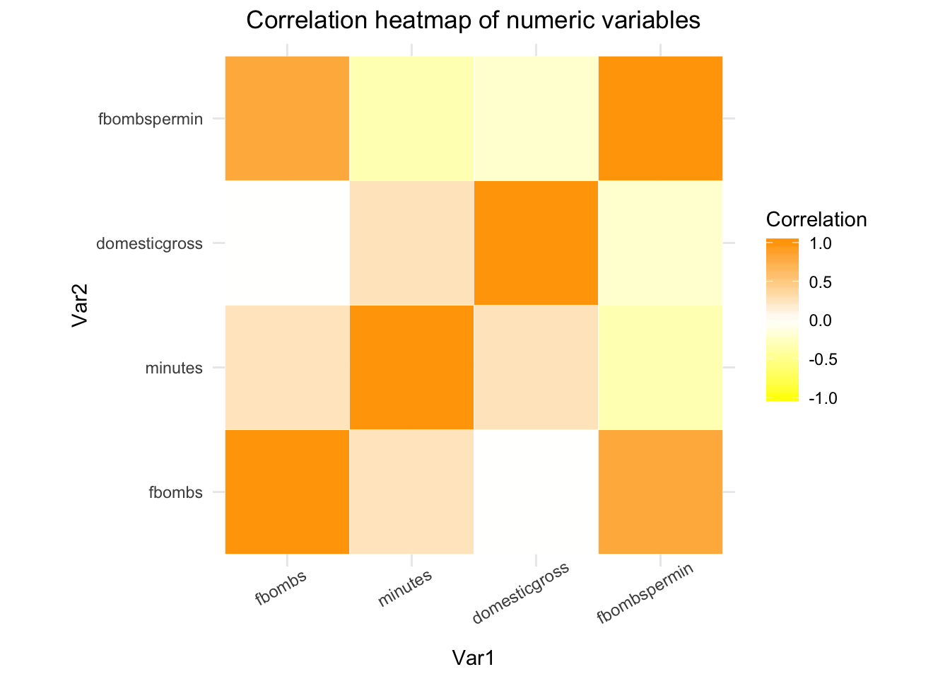

This correlation heatmap takes the correlation matrix coded for summary statistic #8 and converts it into a visualization that makes it easier to see the relationships between the numeric variables. The most positive correlation is shown between ‘fbombs’ and ‘fbombspermin’ while the most negative is shown between ‘minutes’ and ‘fbombspermin’. It was important to use the dplyr select function to not include variables R may have thought were numeric upon inspection such as ‘year’, ‘rank’, and ‘quintileyr’. The fact that there is no correlation between ‘fbombs’ and ‘domesticgross’ makes sense, as all movies are rated R and the audience under the age of 17 is greatly limited. All these movies had a great deal of f-bombs (some much more than others) and this did not correlate with movies doing better or worse when it came to domestic box office sales.

First Plot

bigboys <- filmsdata %>% filter(directorappearances == 4) %>% 
    select(film, director, fbombs, year, fbombspermin)

bigboysgg <- ggplot(bigboys, aes(director, fbombs))

bigboysgg + geom_bar(stat = "identity", aes(fill = film)) + guides(fill = guide_legend(title = "Film", 
    title.position = "left")) + scale_x_discrete(breaks = c("martin.scorsese", 
    "quentin.tarantino", "spike.lee"), labels = c("Martin Scorsese", 
    "Quentin Tarantino", "Spike Lee")) + scale_y_continuous(breaks = seq(from = 0, 
    to = 1600, by = 100)) + ggtitle("Count of Fbombs for Directors with 4 Appearances by Film") + 
    labs(x = NULL) + ylab("Count of Fbombs") + theme_minimal() + 
    theme(plot.title = element_text(hjust = -0.2)) + scale_fill_brewer(palette = "Set3")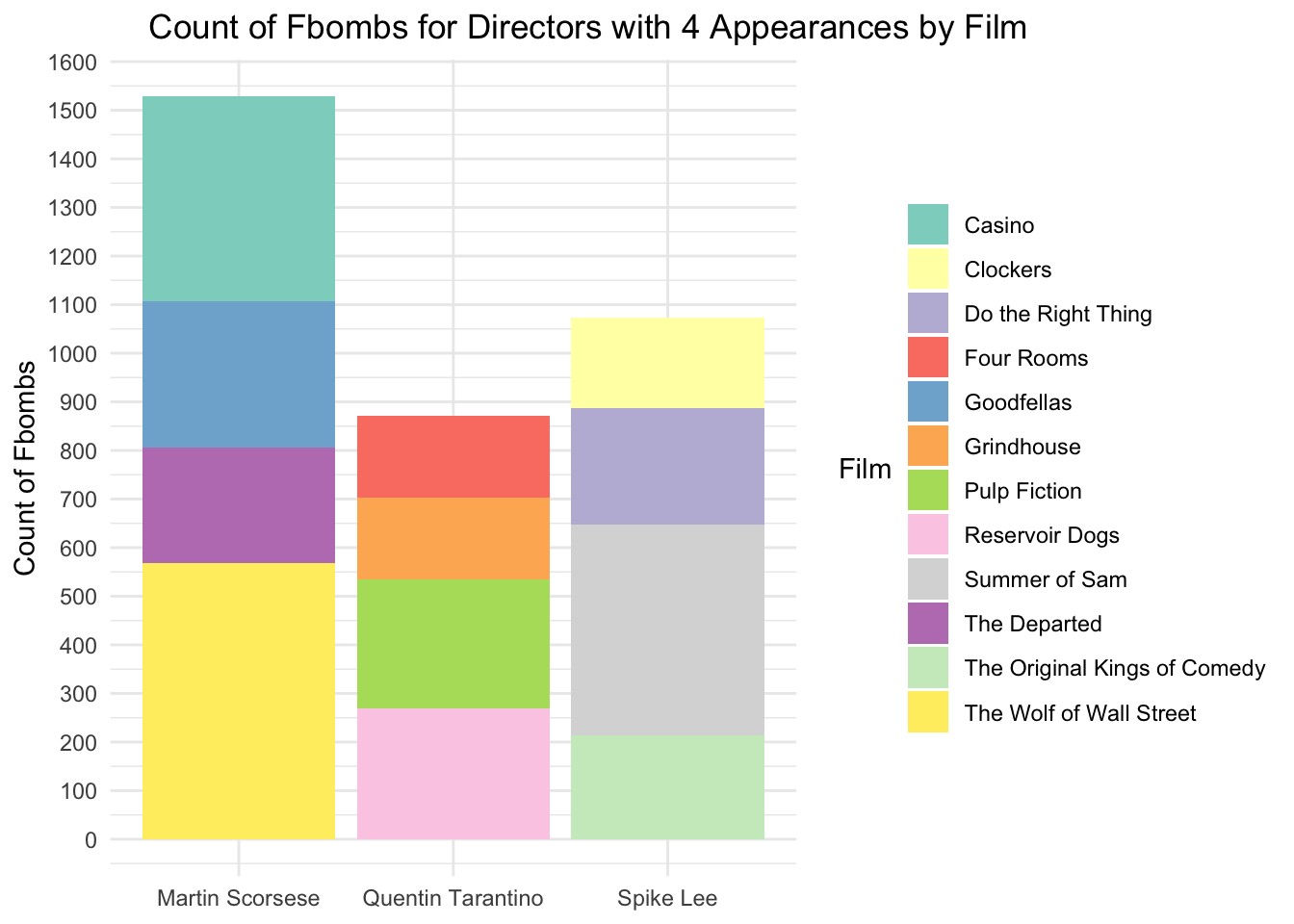

It was interesting to find that out of 132 observations there were three directors that each had four films in the data. Martin Scorsese had the film with the most f-bombs in the dataset (“The Wolf of Wall Street) and Spike Lee has the film with the second most f-bombs in the dataset (”Summer of Sam“). Quentin Tarantino had the lowest combined f-bomb count for his four films when compared to Spike Lee’s and Martin Scorsese’s totals (Martin surpassing Spike Lee by nearly 600 f-bombs!). I found it particularly interesting that Tarantino had two pairs of films in the data with very similar f-bomb totals.”Pulp Fiction" had 265 while “Reservoir Dogs” had 269 and “Grindhouse” had 169 while “Four Rooms” had 168. I wish I could have gotten around to watching “Once Upon a Time in Hollywood” again and while tallying the f-bombs as I watched it to see how it compared to his other four films. If the film ended up having greater than 150 f-bombs (highly likely in a nearly three hour Tarantino film considering his past record) then Tarantino would have been the single director with the most films that made the list at five films total.

Second Plot

complot <- ggplot(filmsdata, aes(x = factor(quintileyr), y = domesticgross)) + 
    geom_bar(stat = "summary", fun.y = "mean", aes(fill = comedy)) + 
    scale_y_continuous(name = "Average Revenue in US Dollars", 
        labels = scales::comma, breaks = seq(from = 0, to = 7e+07, 
            by = 5e+06)) + ggtitle("Average Domestic Box Office Sales per Quintile by Genre") + 
    xlab("Quintile") + ylab("Count of Fbombs") + theme_minimal() + 
    theme(plot.title = element_text(hjust = 0.5)) + scale_fill_brewer(palette = "Set3") + 
    facet_wrap(~comedy)

comedylabels <- c(no = "Non-comedy", yes = "Comedy")

complot + facet_grid(. ~ comedy, labeller = labeller(comedy = comedylabels)) + 
    theme(legend.position = "none") + scale_x_discrete(breaks = c("[1978,1997]", 
    "(1997,2000]", "(2000,2006]", "(2006,2012]", "(2012,2019]"), 
    labels = c("1978-97", "1998-00", "2001-06", "2007-12", "2013-19")) + 
    theme(axis.text.x = element_text(angle = 27, vjust = 0.5))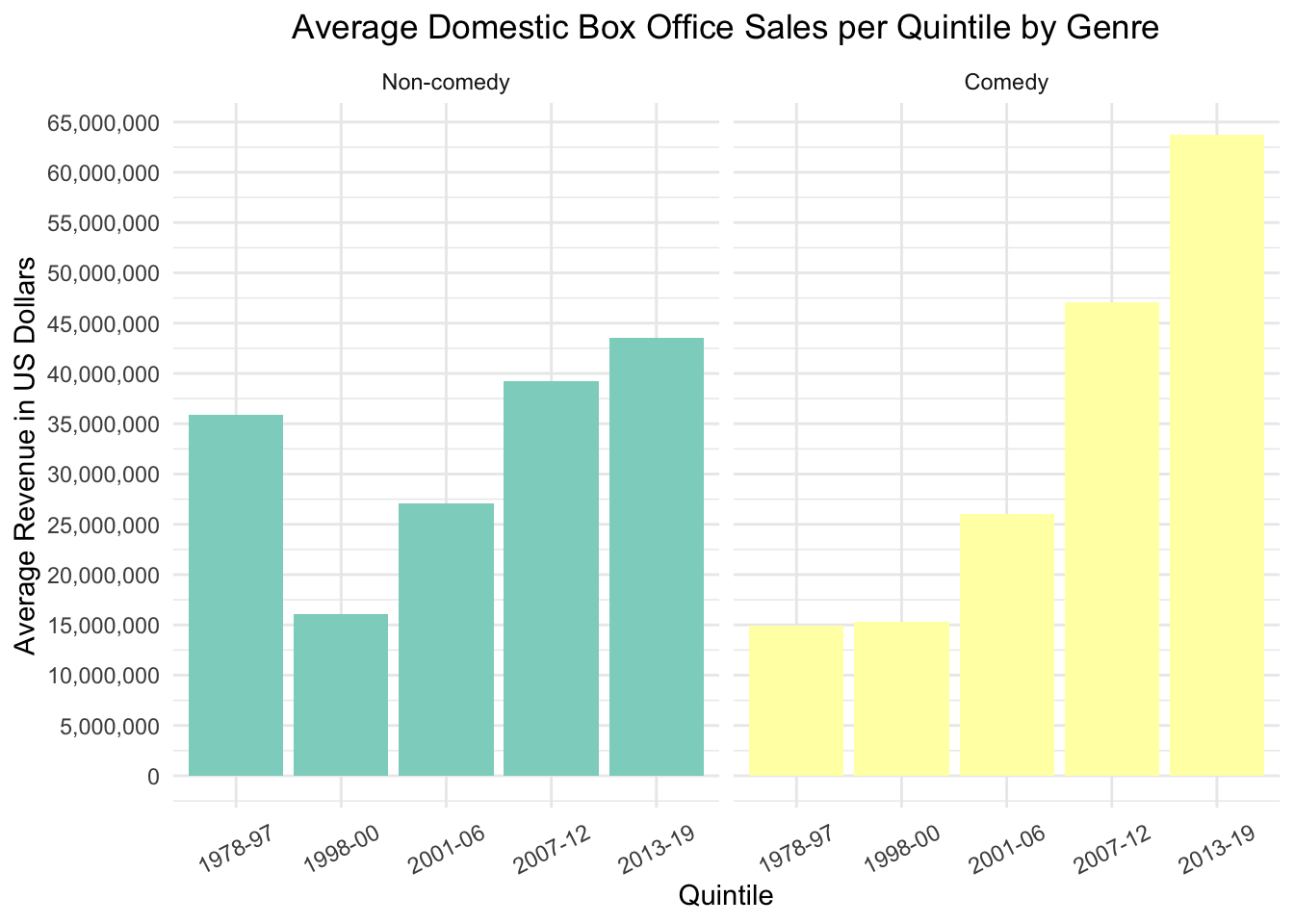

This plot shows how the comedies compare to the non-comedies when average domestic box office sales is concerned, based on quintile. I made the quintiles to better compare observations as otherwise it would simply be a plot of each year’s average revenue (in some cases just being the revenue one movie brought in rather than a true average since it was the only one for a particular year). Forming five quintiles from the years made it more intuitive to see which range of years brought in the most revenue for these highly vulgar movies. As one can see the fifth quantile has the highest average revenue in both the comedy and non-comedy groups. This may partly be due to the top 3 grossing films in the dataset being from the fifth quartile (“22 Jump Street”, “Straight Outta Compton”, and “The Heat”), but making five quintiles allows for a better assessment of average revenue than if one were to divide the years into 10 quintiles for such a small dataset. The non-comedies consisting of action films, dramas, crime films, etc. on average did better in the box office than the comedies until after 2006. Another interesting trend is that the average revenue for the non-comedies in first quintile starts strong, but tapers off or remains close to the first quintile in later years. The comedies on the other hand always show a considerable increase in average revenue as the quintiles proceed to 2013-2019, the quintile with highest revenue in the comedy group as well as when compared to the non-comedies.

Clustering

library(cluster)
filmsclust <- filmsdata %>% select(fbombs, minutes, domesticgross, 
    fbombspermin)
sil_width <- vector()
for (i in 2:10) {
    pam_fit <- pam(filmsclust, k = i)
    sil_width[i] <- pam_fit$silinfo$avg.width
}
ggplot() + geom_line(aes(x = 1:10, y = sil_width)) + scale_x_continuous(name = "k", 
    breaks = 1:10)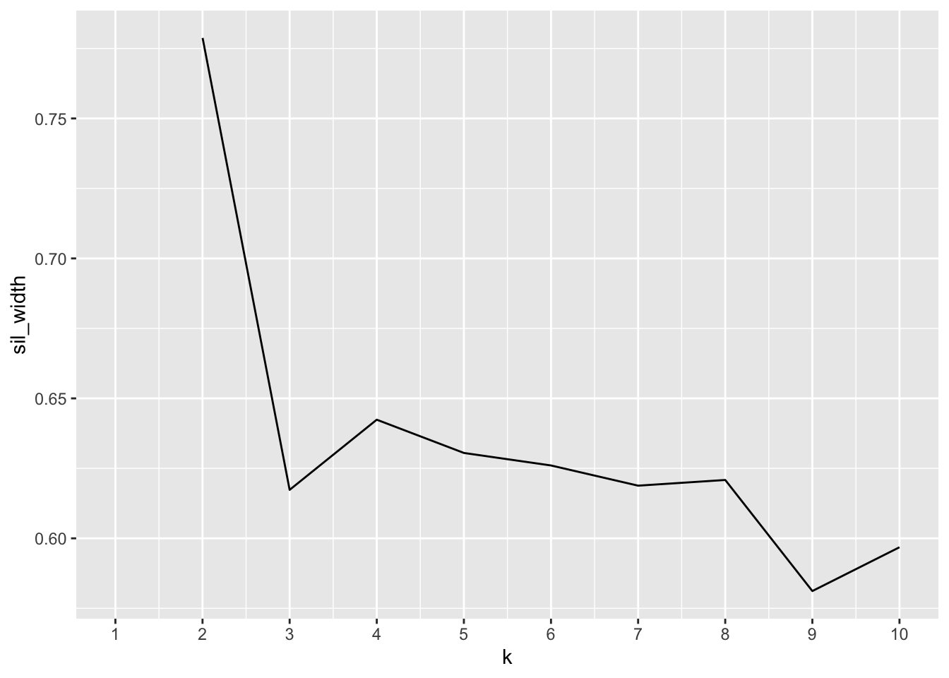

pamfilms <- pam(filmsclust, k = 2)
silpam <- silhouette(pamfilms)
plot(silpam)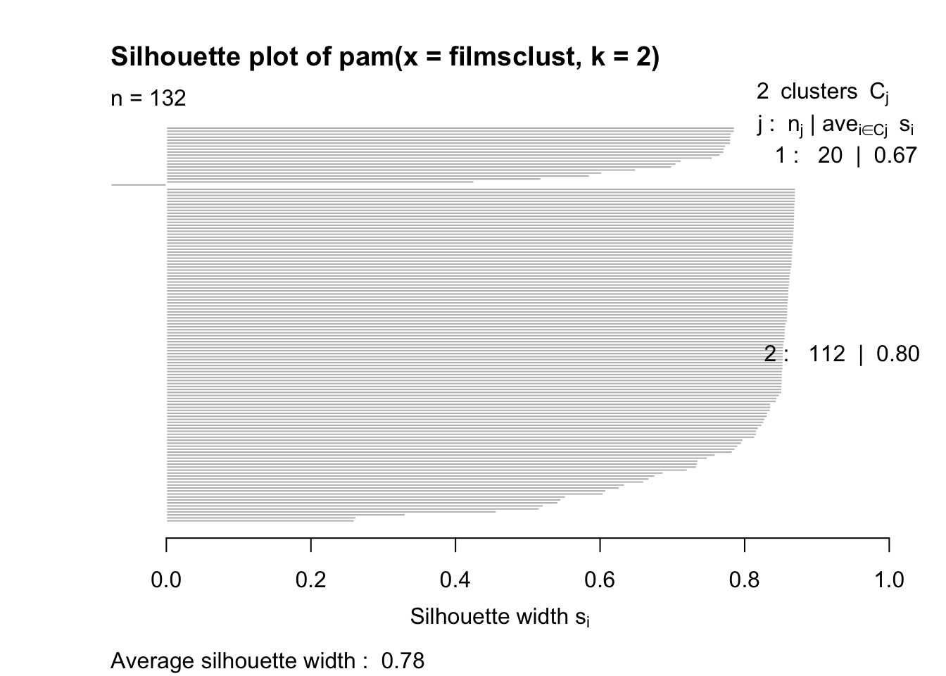

finalfilmsclust <- filmsdata %>% mutate(cluster = as.factor(pamfilms$clustering))
ggplot(finalfilmsclust, aes(x = domesticgross, y = fbombspermin, 
    color = cluster)) + geom_point()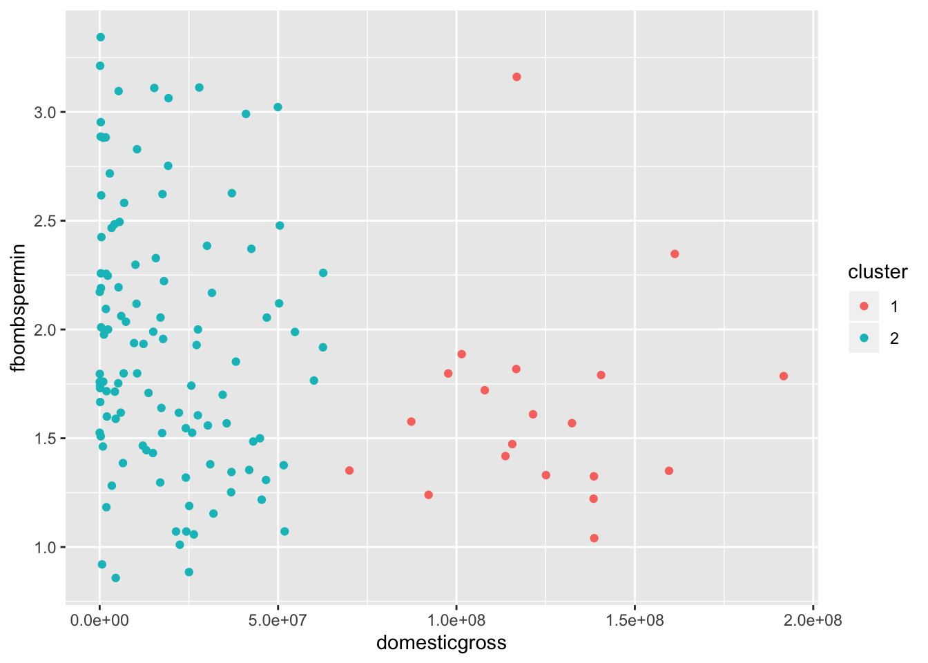

library(GGally)
finalfilmsclust %>% select(fbombs, minutes, domesticgross, fbombspermin, 
    cluster) %>% ggpairs(columns = 1:4, aes(color = cluster))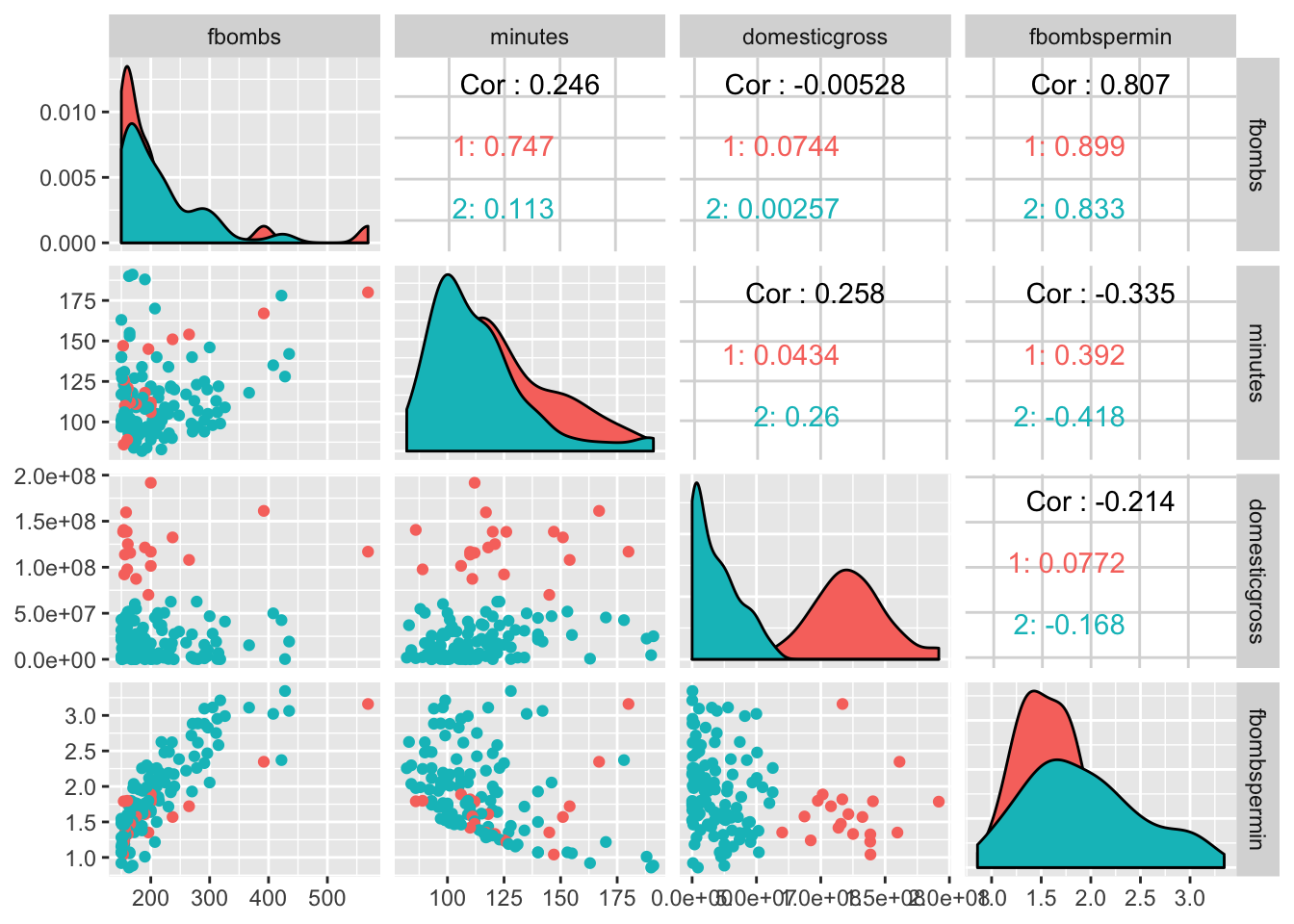

After performing PAM and kmeans clustering, I found out the two clustered the data quite differently. I went with PAM as the clusters seemed more distinct for the variables at hand. After making a new dataframe only containing the numeric variables of interest (fbombs, minutes, domesticgross, and fbombspermin), sil_width showed it made the most sense to cluster into two after analysis of the plot.When viewing the separate silhouette plot, PAM clustering showed there was strong structure (average silhouette width = 0.78) to be found between the two clusters, so most of the values belonged to the clusters they were assigned.

The ggpairs package provided a nice cohesive summary all in one chart, separated into several boxes based on information about correlations between two variables concerning the clusters. The the number of f-bombs in a film was shown to almost have much no correlation to the domestic box office sales. So increased cursing in a film did not correlate with increased revenue or vise versa, which makes sense since all these films are rated R and the target audience is greatly limited to adults. The highest positive correlation was seen between ‘fbombspermin’ and ‘fbombs’. Both cluster 1 and 2 exhibited this with values at 0.89 and 0.83 respectively. This also makes sense because the more f-bombs a film has is going to directly correlate with more f-bombs that film has per minute.

Taking information gathered from the ggpairs analysis, plotting with ggplot based on x = ‘domesticgross’ and y = ‘fbombspermin’ was performed as the clusters appeared the most separated and the two variables compared the most relevant. After looking at the ggplot as well as the data itself (arranging descending by variable) for the dataframe with the now included clusters it was apparent that clustering was largely based on how well the film did at the box office. Having a relatively small dataset made understanding and comprehension the data very manageable, as direct films could easily be found from cluster 2. It was really neat to find out with exceptions that most of the top grossing films ended up having only a moderate amount of f-bombs per minute when compared to many from cluster 2. Of course outliers such as “The Wolf of Wall Street” and “Straight Outta Compton” ended up doing exceptionally well despite the frequency of the word, but these are the only 2 out of 20 that showed this difference in cluster 1. Of course all 132 of these films had tons of vulgar language as they were the ones that made the “List of films that most frequently use the word”f$#%", but nevertheless it was a fun time exploring the several differences and similarities between them.